
From a Prompt to a Validated Solver: Fermioniq's Sofia Brings Agent-Built Physics to NVIDIA GPUs
Sofia is a solver factory: an agentic simulation expert with its own toolkit and domain-specific language (DSL) for producing physics simulations. An engineer - or agent - states a task in plain language. Sofia's agent chooses the physics, writes the solver, debugs and validates it, and hands back a solver a human can read and verify. Sofia compiles that solver into NVIDIA Warp kernels and JAX control flow for GPU-native execution. In a water-modelling case-study with Deltares and the Ministry of Infrastructure and Water Management, the Sofia agent took less than half an hour to build a validated, GPU-accelerated simulation of the river Waal.
By Fermioniq, in collaboration with NVIDIA · featuring a case study with Deltares and the Ministry of Infrastructure and Water Management.
Often the bottleneck is not running the solver, but writing it
GPUs are making large simulations cheaper to run. What still costs weeks is everything around the run: choosing a numerical method and discretisation scheme, writing it out by hand, debugging that one sign error that produced a plausible but wrong answer, and then validating the solver in various scenarios before the result can be trusted. To make things worse, existing solvers are often deeply embedded in legacy software written for CPUs, and porting that code to run on GPUs is a multi-million euro refactor.
AI agents offer a path forward. But so far the right tools and languages for writing physics simulations have been missing. A general-purpose array framework asks agents to get indexing, staggering, boundary handling and memory layout right at the same time as the physics, all the while tuning everything for efficient GPU execution. The resulting code is often expensive to generate, impossible to maintain, and cannot pass the crucial step of human verification that is required by the end users.
Fermioniq's Sofia solves these challenges by bringing the right tooling for agentic physics simulation. The Sofia DSL (Domain Specific Language) provides the right level of abstraction for designing physics simulations: mathematics. The Sofia agent draws on a base of domain-specific knowledge, deep understanding of the Sofia DSL, and previous experience to rapidly produce bespoke simulations in the Sofia DSL.
Sofia: a simulation-expert agent with its own DSL for physics
The Sofia DSL (Domain Specific Language) provides the right level of abstraction for designing physics simulations: mathematics. The Sofia agent draws on a base of domain-specific knowledge, deep understanding of the Sofia DSL, and previous experience to rapidly produce bespoke simulations in the Sofia DSL.
Sofia DSL and code generation
The Sofia DSL describes a simulation at the level of the equations, building on the popular Python library Sympy, so the interface feels familiar. Fields are continuous. A conservation law is written as du/dt = F(u, ∇u, …) using operators such as diff, laplacian and divergence. Derivative stencils, boundary conditions, and time-stepping schemes are lowered automatically into discrete forms. Every level of lowering is directly accessible, meaning that discrete methods such as lattice-Boltzmann can be expressed in the same language. Boundaries, staggered grids, and geometries from CAD are first-class citizens. Sofia's code generation layers deterministically turn symbolic expressions into concrete array operations, apply staggering, boundary conditions and optimisations such as CSE. The code generation emits per-cell updates as NVIDIA Warp kernels, with the control flow, JIT compilation, reductions and gradients handled by JAX. All of this is only made possible by the interoperability of Warp and JAX.
Because the physics is written at the level of the equations, a solver program is short and easy for a modelling expert to read. An incompressible Navier–Stokes solver with a penalised body and a far-field fringe is twelve lines of equations in Sofia. Written directly as Warp kernels, the same solver needs the derivative stencils, the staggered indexing, the boundary conditions and ghost cells, the projection step and the Runge–Kutta staging all spelled out by hand, which runs to several hundred lines of kernel code. This difference has the most impact when the physics changes. Adding a term to the momentum equation or swapping the advection scheme is a one-line change in Sofia. In hand-written kernels it requires a rewrite of every kernel that touches that field, plus a new round of debugging and validation.
# Incompressible Navier–Stokes in Sofia: penalised body, far-field fringe, projection
G = Grid(ndim=2)
x, y = G.coordinates
u, v, p = (Field(n, domain=G) for n in ("u", "v", "p"))

def rhs(a, a_free):
    return (-u * diff_upwind(a, x, variable=u) - v * diff_upwind(a, y, variable=v)
            + nu * laplacian(a)            # viscous
            - chi * a / eta                # no-slip by Brinkman penalisation
            - sig * (a - a_free))          # far-field fringe

step = ir.RKn(F={u: rhs(u, U0), v: rhs(v, 0.0)}, order=3, dt=dt,
              post=ir.ProjectDivFree((u, v), p))
sim = backend.jit(build_simulation(code, specs, kernel_backend="warp"))
Sofia agent
Sofia ships with an agent harness. The agent knows which physics to apply for a given simulation task and which numerical schemes best suit it. It knows how to build and run a Sofia simulation, how to read the result, and what common failure modes to look for. It runs the solver and validates things such as conservation, boundary behaviour and grid convergence. What it hands back is not a black-box solver with opaque physics, but a validated solver written in the Sofia DSL, short enough for the engineer who asked for it to read, review and change.
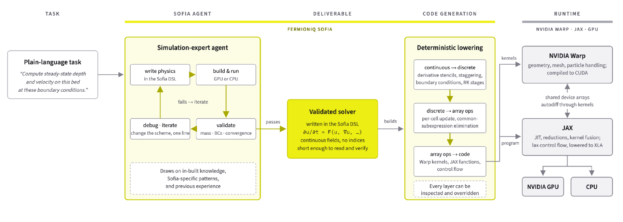 Figure 1. The Sofia pipeline. The agent iterates on a solver written in the Sofia DSL until it passes validation, then delivers a solver package. Sofia generates Warp kernels for the cell updates, geometry handling, and meshing, with JAX code for control flow, targeting NVIDIA GPUs or a CPU from the same script.
How NVIDIA Warp accelerates Sofia
Sofia does not have its own GPU runtime: it lowers operations to NVIDIA Warp kernels and JAX functions, and orchestrates them with JAX. The geometry, meshing, and particle simulation pipelines of Sofia build on the components offered by the Warp framework. The Warp/JAX interoperability means that features such as auto-differentiation through a full solve work out of the box.
Engineering problems usually arrive with CAD models. Warp's mesh data structures and methods such as closest-point and signed-distance queries let Sofia handle complex geometries without leaving the GPU, enabling GPU-native implementations of techniques required for modern physics simulation such as wall modelling in computational fluid dynamics.
What this means for our customers
Deltares and the Ministry of Infrastructure and Water Management use-case: simulation of the river Waal
One domain where Sofia can have an impact is water modelling: the simulation of rivers, lakes, estuaries, and coastal areas. Recent years have shown, all too often, how devastating floods and storm surges can be. And as climate change drives more extreme weather events, such disasters are becoming more common. The ability to model these water systems quickly and accurately, across a wide range of conditions, is one of the first steps in preparing for such events and limiting the damage they can cause.
It's perhaps no surprise that one of the world leaders in this field is Dutch. Around a quarter of the Netherlands lies below sea level, with much of the rest at constant risk of flooding without carefully applied water management. Deltares, an independent Dutch research institute, develops much of the modelling software behind that effort, such as the Delft3D and D-HYDRO suites.
The Ministry of Infrastructure and Water Management, the national water authority, uses these models and software to manage the country's critical water infrastructure. That expertise is used around the world, from flood forecasting in North America to flood and coastal resilience across Asia.
Experience has taught us that an ageing infrastructure, a changing climate and a growing demography of the Netherlands require us to continuously increase the detail and accuracy levels of our numerical models, which in turn translates into an increase in computational cost. We develop, use and maintain several hundreds of complex numerical models for physics simulations, and are looking for ways to significantly reduce the runtimes, costs, and computational requirements of our current simulation workloads. — a representative of the Ministry of Infrastructure and Water Management.
Staying ahead of these challenges means continually building new models: adapting solvers to incorporate new physics, new geometries, and new questions as requirements change. Having tested Sofia on a model of the Waal, Dr. Hans Putten, Director of Digital Strategy at Deltares, expects that with Sofia, "the development of the solver and associated applications can be reduced from the order of days to the order of a few hours compared to our current approach".
The Waal is the main distributary of the Rhine in the Netherlands. It carries about two thirds of the Rhine's flow and is the principal shipping route between the port of Rotterdam and Germany. In this use-case, which was originally part of a larger research project, the task was to use Sofia to compute the steady-state water depth and velocity along an 85 km length of the Waal under typical flow conditions. The river bed arrives as a bathymetry grid of 2.3 million cells at 25 m resolution.
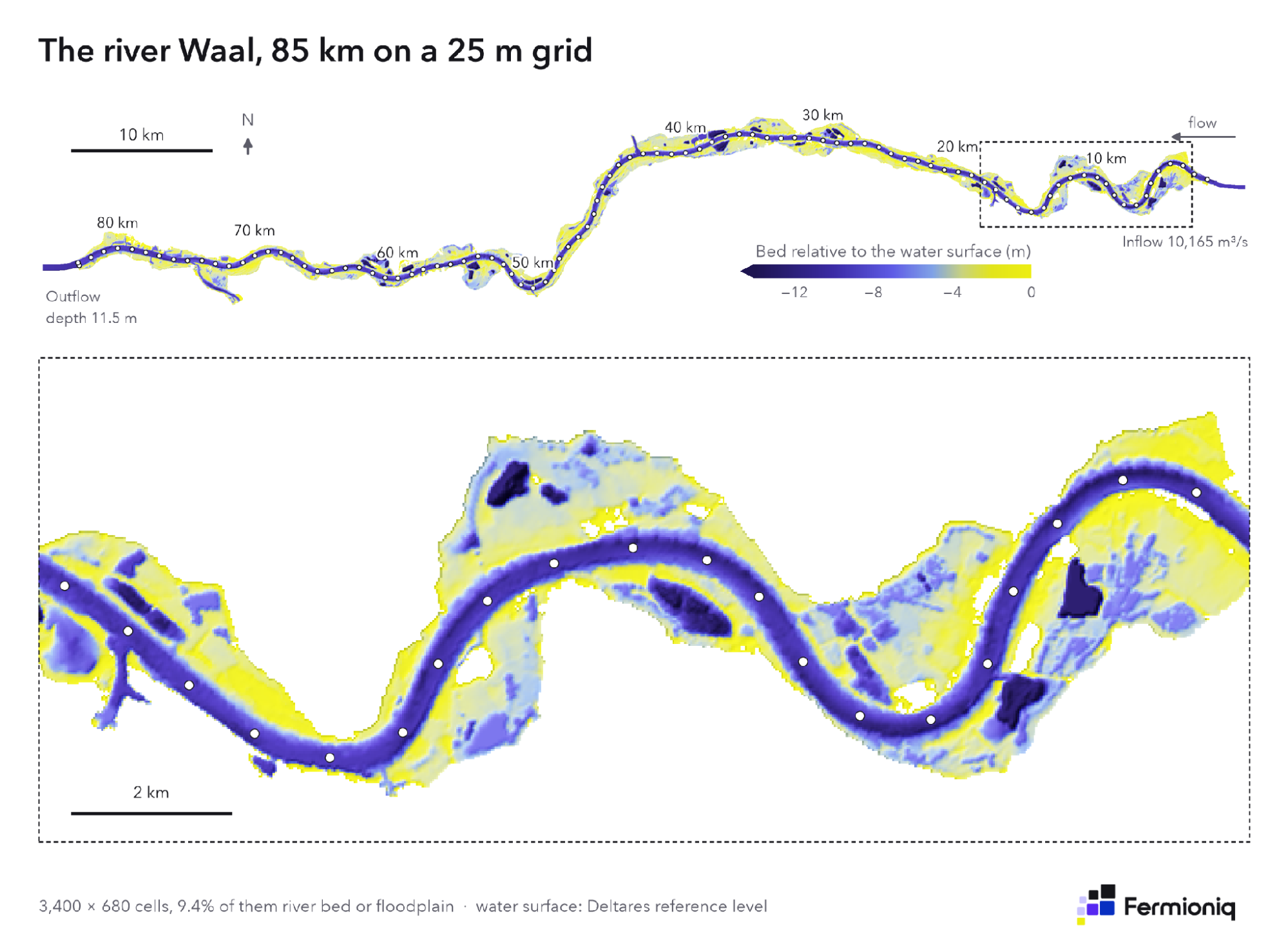 Figure 2. The 85 km river and segment on the 25m grid, with the river flowing east to west. The bed is coloured by its height relative to the water surface. The dots are the 96 observation points where solutions are compared with Deltares' reference.
A hand-built solver in Sofia
We hand-built a solver in the Sofia DSL, and verified and validated it together with the modelling experts at Deltares, a task made easier by the high-level interface. The outcome was a solver that matched Deltares' reference data on the problem to within 40cm on observation points across the length of the river.
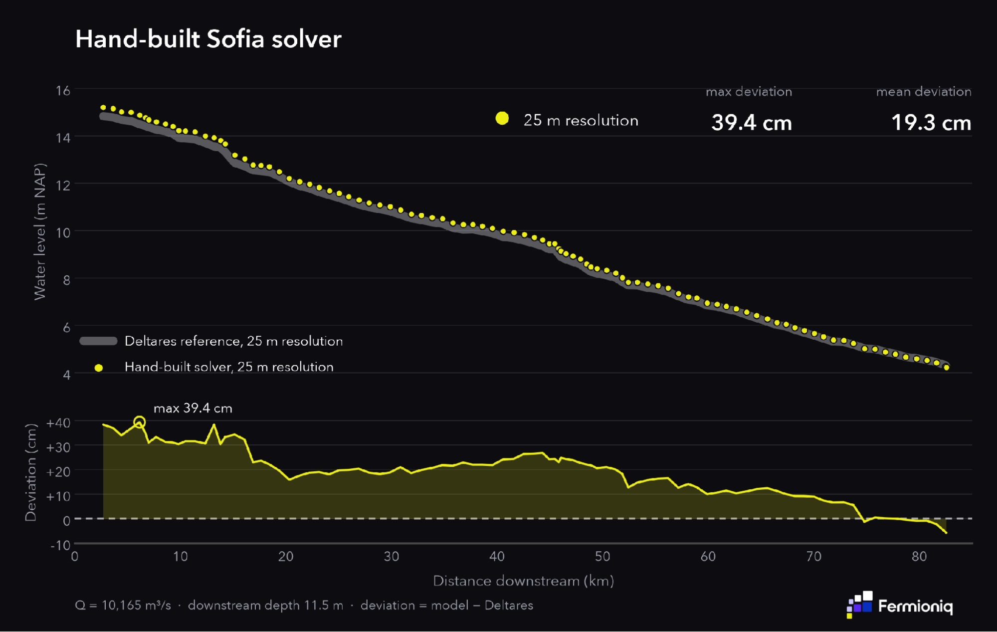 Figure 3. Water level from the hand-built Sofia solver at the observation points, over the Deltares reference, with the deviation from it below. Water level is above NAP (Normaal Amsterdams Peil) - essentially an average of the North Sea level.
With GPU acceleration, the runtime per-update step was competitive with Deltares' own software.
To demonstrate the saving in complexity obtained by using Sofia, at the end of the post we show (part of) a Warp kernel implementing the x-momentum update term for a simulation, generated by Sofia. Below that is the Sofia code that generated it. The entirety of the generated code is almost 600 lines. The Sofia program is just 46.
The Sofia agent's solver
The real benefit of Sofia comes with the Agentic layer attached. We gave the Sofia agent the same task: compute the steady-state depth and velocity on this bed at these boundary conditions. We deliberately left the choice of numerical method to the agent. The task fixed the equations, the bed, and the boundary conditions but said nothing about discretisation, time integration or how to reach steady state, so that the agent could suit the scheme to the problem and to Sofia rather than follow a strict template.
Within 30 minutes, and only €1.87 of tokens spent, the agent returned a new solver which outperformed our hand-written one.
It tested several numerical schemes for river flow; tried two flooding-and-drying treatments and measured the difference in conveyance; checked whether a background eddy viscosity was needed to settle the deep scour pits in the bed. Each test was a short Sofia script, a run, and a check. Finally, it settled on a method, validated it with standard tests (mass conservation, boundary condition satisfaction, grid refinement, and various sanity checks), and returned the solver as a deliverable.
The solver performed better on Deltares' validation data than the solver we had built by hand, with less than 13cm deviation across all observation points at the usual 25m cell resolution. Remarkably, the solve was still accurate at 50m resolution (avg. deviation 6.5cm -> 7.1cm; max. deviation 12.7cm -> 22.1cm): resulting in a run with 25% of the memory footprint of the original. At that resolution, our hand-built solver performed markedly worse.
Contrast this process to the one we took at the start of the project: as method experts, with Deltares on hand with modelling expertise, it took us a number of months to build a solver, and over a year to get it to the point where it agreed with Deltares' software, which itself was built by deep domain experts over decades. This process was shortened to weeks with a precursor to Sofia, and now to minutes with the Sofia agent.
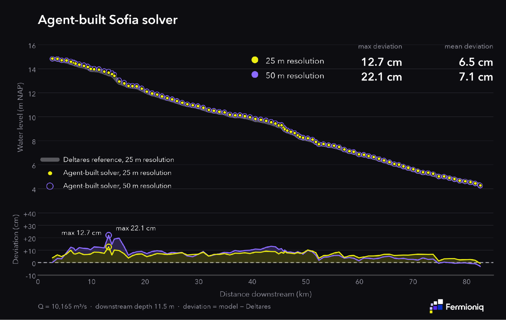
Figure 4. The same comparison for the agent-built solver, at 25 m and 50 m resolution. Water level is above NAP (Normaal Amsterdams Peil) - essentially an average of the North Sea level.
The solver methodology can be easily inspected by domain experts by simply inspecting the Sofia code that it generated:
# Shallow-water momentum and continuity on a C-grid, as written by Sofia's agent
zeta = Field("zeta", domain=grid)
u = Field("u", domain=grid, staggered=Staggered.XFACE)
v = Field("v", domain=grid, staggered=Staggered.YFACE)

wet_u = hu**2 / (hu**2 + H_MIN**2)                      # flooding-and-drying weight
speed = sp.sqrt(u*u + v*v + 1e-12)

f_u = (wet_u * (-u * diff_upwind(u, x, variable=u) - v * diff_upwind(u, y, variable=v)
                - GRAV * diff(zeta, x) + NU_H * laplacian(u))
       - CF * u * speed / sp.Max(hu, H_FRIC)             # bed friction, c_f fixed
       - (1 - wet_u) * u * r_dry)                        # relax dry faces to rest
f_z = (-diff(hu * u, x, allow_expand=False)              # flux form: mass telescopes
       - diff(hv * v, y, allow_expand=False))

step = ir.RKn({zeta: f_z, u: f_u, v: f_v}, order="SSPRK3", dt=dt, post=boundary_pins)
sim  = build_simulation(code, specs, kernel_backend="warp")
Code complexity reduction from Sofia
Below is part of a Warp kernel for one part of a simulation, generated by Sofia. This is the type and length of code that would need to be written, maintained, and verified by experts (or coding agents) building a simulation. Below it is the Sofia code that generated it.
@warp.kernel
def kernel_impl_3907048(
    v_s_1: warp.array2d[warp.float64],
    v_s_0: warp.array2d[warp.float64],
    zeta_s_2: warp.array2d[warp.float64],
    zeta_s_1: warp.array2d[warp.float64],
    zb: warp.array2d[warp.float64],
    zeta_s_0: warp.array2d[warp.float64],
    v_s_2: warp.array2d[warp.float64],
    u_s_2: warp.array2d[warp.float64],
    u_s_0: warp.array2d[warp.float64],
    u_s_1: warp.array2d[warp.float64],
    u_3906986: warp.array2d[warp.float64],
):
    i, j = warp.tid()
    x0 = zeta_s_0[i, j]
    x1 = zeta_s_1[i, j]
    x2 = zeta_s_2[i, j]
    x3 = zeta_s_0[((1) + (i)) % 204, j]
    x4 = zeta_s_1[((1) + (i)) % 204, j]
    x5 = zeta_s_2[((1) + (i)) % 204, j]
    x6 = u_s_0[i, j]
    x7 = u_s_1[i, j]
    x8 = u_s_2[i, j]
    x9 = u_s_0[((1) + (i)) % 204, j]
    # ... x10-x27: 18 more stencil reads, face-averaged v, upwind coefficients
    u_3906986[i, j] = (
        ((warp.float64(0.998096209169431)) * (x6))
        + ((warp.float64(0.000475947707642355)) * (x10))
        + ((warp.float64(0.000475947707642355)) * (x11))
        + ((warp.float64(0.000475947707642355)) * (x12))
        # ... 17 more terms: RK3 weights (1/6, 4/6, 1/6) x viscosity and pressure gradient
        + (
            (warp.float64(-0.0951895415284710))
            * (x22)
            * (
                (
                    (
                        ((warp.float64(-1)) * (x25))
                        + ((warp.float64(0.200000000000000)) * (x11))
                        + (
                            (warp.float64(-0.0500000000000000))
                            * (u_s_0[i, ((2) + (j)) % 44])
                        )
                    )
                    if (x22 < warp.float64(-0.00000100000000000000))
                    else (
                        (
                            (x25)
                            + (
                                (warp.float64(0.0500000000000000))
                                * (u_s_0[i, ((-2) + (j)) % 44])
                            )
                            + ((warp.float64(-0.200000000000000)) * (x12))
                        )
                        if (x22 > warp.float64(0.00000100000000000000))
                        else (
                            ((warp.float64(0.0500000000000000)) * (x11))
                            + ((warp.float64(-0.0500000000000000)) * (x12))

                )
            )
        )
        # ... 227 more lines: the other five upwind switches, bed friction

)
                    )
This was a small fraction of the code generated from the Sofia code, which defines the full simulation:
G = Grid(ndim=2, boundaries=((GH - 0.5, -(GH - 0.5)), (GH - 0.5, -(GH - 0.5))))
x, y = G.coordinates
zeta = Field("zeta", domain=G)
u = Field("u", domain=G, staggered=Staggered.XFACE)
v = Field("v", domain=G, staggered=Staggered.YFACE)
zb = Field("zb", domain=G)
h = zeta - zb

def momentum(a, dx_):
    return (-u * diff_upwind(a, x, variable=u) - v * diff_upwind(a, y, variable=v)
            - G_ACC * diff(zeta, dx_)
            + NU * laplacian(a)
            - CF * a * sp.sqrt(u**2 + v**2) / sp.Max(h, H_MIN))

F = {zeta: -diff(h * u, x, allow_expand=False) - diff(h * v, y, allow_expand=False),
        u: momentum(u, x),
        v: momentum(v, y)}

start_x, end_x = sp.Eq(x, G.DomainStart), sp.Eq(x, G.DomainEnd)
start_y, end_y = sp.Eq(y, G.DomainStart), sp.Eq(y, G.DomainEnd)
bcs = ir.CodeBlock(
    apply_boundary_conditions(((sp.Eq(diff(zeta, x), 0), start_x),
                                (sp.Eq(zeta, Z_OUT), end_x),
                                (sp.Eq(diff(zeta, y), 0), start_y),
                                (sp.Eq(diff(zeta, y), 0), end_y)),
                                field=zeta, as_eval_assignment=True),
    apply_boundary_conditions(((sp.Eq(u, Q_IN / sp.Max(h, H_MIN)), start_x),
                                (sp.Eq(diff(u, x), 0), end_x),
                                (sp.Eq(diff(u, y), 0), start_y),
                                (sp.Eq(diff(u, y), 0), end_y)),
                                field=u, as_eval_assignment=True),
    apply_boundary_conditions(((sp.Eq(diff(v, x), 0), start_x),
                                (sp.Eq(diff(v, x), 0), end_x),
                                (sp.Eq(v, 0), start_y),
                                (sp.Eq(v, 0), end_y)),
                                field=v, as_eval_assignment=True))

code = ir.CodeBlock(
    ir.Inputs((zeta, u, v, zb)),
    bcs,                                   # fill the ghosts before the first stage
    ir.For(length=nsteps, body=ir.RKn(F=F, order=3, dt=DT, post=bcs)),
    ir.Outputs((zeta, u, v)))
shape = (NX + 2 * GH, NY + 2 * GH)
specs = {G: dict(shape=shape, extent=((0.0, NX * DX), (0.0, NY * DX)))}
sim = build_simulation(code, specs, kernel_backend="warp")
What comes next
The Fermioniq-Deltares collaboration continues with the development and benchmarking of 3D water simulations. We have already hand-built and validated a 3D solver in Sofia, and are actively identifying opportunities to deploy Sofia on a broader range of computationally-heavy models used by Deltares and the Ministry of Infrastructure and Water Management..
As for Sofia itself, the next releases will see the addition of:
- Particle-based methods. Allowing simulation methods such as Smooth Particle Hydrodynamics (SPH), and coupling of these to continuum methods. These will be built on Warp's particle and hash-grid primitives so that neighbour search and particle-to-grid transfer run on the GPU without leaving the Sofia program.
- Mesh refinement. Adaptive refinement built on Warp's sparse volume and spatial data structures, increasing the scale and accuracy of simulations that can be run in Sofia.
- An ever improving agent. The knowledge base and skill set of the Sofia agent continues to grow together with the Sofia DSL, opening up new types of physics and simulation domains.